LRP
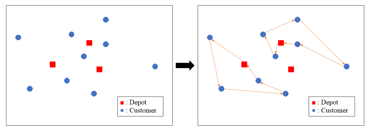
Location Routing Problem (LRP) is a combination problem of Location Allocation Problem and Vehicle Routing Problem. The goal of the LRP is determining the location of depots and the routes of the vehicles for serving the customers which minimize the total cost. This post solves the LRP with Integer Linear Programming using Python.
1
2
3
4
5
from mip import Model, xsum, minimize, BINARY
import matplotlib.pyplot as plt
import pandas as pd
import numpy as np
import itertools
Problem definition
There are randomly generated 15 nodes comprised with 5 depot nodes and 10 customer nodes. The numbers in the list represent x-coordinate, y-coordinate, demand, capacity and opening cost. Note that the depot nodes don’t have any demand and also the customer nodes don’t have any capacity and opening cost. The opening cost of all depot is 100. The fixed cost for a vehicle is 10. The traveling cost is Euclidean distance of route.
1
2
3
4
5
6
7
8
9
10
11
12
13
14
15
16
# [geo_x, geo_y, demand, capacity, opening cost]
nodes = [[ 69.7234,  20.2083,   0.0000, 101.0000, 100.0000],
         [ 30.2384,  43.5044,   0.0000, 101.0000, 100.0000],
         [ 61.9749,   6.9667,   0.0000, 101.0000, 100.0000],
         [ 99.0928,  30.2991,   0.0000, 101.0000, 100.0000],
         [ 82.4491,  39.9930,   0.0000, 101.0000, 100.0000],
         [ 28.8304,  62.9077,   9.0000,   0.0000,   0.0000],
         [ 47.4790,  73.0949,  18.0000,   0.0000,   0.0000],
         [ 82.1459,  44.1756,   7.0000,   0.0000,   0.0000],
         [ 21.9554,  60.2978,   3.0000,   0.0000,   0.0000],
         [ 47.1047,   8.9509,   3.0000,   0.0000,   0.0000],
         [ 72.2547,  29.8323,  19.0000,   0.0000,   0.0000],
         [ 67.7186,  84.6980,  14.0000,   0.0000,   0.0000],
         [ 74.1557,  69.2824,   9.0000,   0.0000,   0.0000],
         [ 20.8579,  59.8875,   1.0000,   0.0000,   0.0000],
         [ 82.8111,  10.4402,  18.0000,   0.0000,   0.0000]]
Set
$I$ represents list of the depot nodes.
$J$ represents list of the customer nodes.
$V$ represents list of all nodes.
$K$ represents list of vehicles.
$S$ represents list of all subset of $J$ excepting null set.
1
2
3
4
5
6
7
8
9
10
11
12
13
14
15
16
17
18
19
20
21
22
23
24
25
geo = []
depot = []
customer = []
distance = {}

for node in nodes:
    geo.append((node[0], node[1]))
    if node[2] == 0:
        depot.append(node)
    else:
        customer.append(node)

for i in range(len(geo)):
    for j in range(len(geo)):
        distance[(i,j)] = np.linalg.norm(np.array(geo[i])-np.array(geo[j]))

I = list(range(len(depot)))
J = list(range(len(depot), len(customer)+len(depot)))
V = list(I+J)
K = [1, 2, 3, 4, 5]

print(I)
print(J)
print(V)
print(K)
1
2
3
4
[0, 1, 2, 3, 4]
[5, 6, 7, 8, 9, 10, 11, 12, 13, 14]
[0, 1, 2, 3, 4, 5, 6, 7, 8, 9, 10, 11, 12, 13, 14]
[1, 2, 3, 4, 5]
1
2
3
4
5
6
7
8
9
10
11
12
def subset(node_list):
    subset_list = []

    for iter in range(len(node_list)):
        if iter != 0:
            iter_subset_list = list(itertools.combinations(node_list, iter))
            for sub in iter_subset_list:
                subset_list.append(list(sub))

    return subset_list

S = subset(J)
Following code shows how nodes are distributed.
1
2
3
4
5
6
7
8
9
10
11
12
13
14
15
16
17
18
19
20
21
22
depot_x = [node[0] for node in depot]
depot_y = [node[1] for node in depot]
customer_x = [node[0] for node in customer]
customer_y = [node[1] for node in customer]
depot_number = 0
customer_number = 5

plt.figure(figsize=(12,8))
plt.scatter(depot_x, depot_y, c="red", marker="*", s=100, label="depot")
for depot_node in depot:
    plt.text(depot_node[0]-0.5, depot_node[1]+1, str(depot_number), fontsize=12)
    depot_number += 1
plt.scatter(customer_x, customer_y, c="green", marker="^", s=100, label="customer")
for customer_node in customer:
    if customer_number >= 10:
        plt.text(customer_node[0]-1, customer_node[1]+1, str(customer_number), fontsize=12)
        customer_number += 1
    else:
        plt.text(customer_node[0]-0.5, customer_node[1]+1, str(customer_number), fontsize=12)
        customer_number += 1
plt.legend()
plt.show()

Following mathematical formulation is referred to Vincent et al. (2010).
1
m = Model()
Variables and Parameters
Decision variable
$x_{ijk}$ is a binary variable whether the node $i$ and the node $j$ are directly connected by vehicle $k$.
$y_i$ is a binary variable whether the depot node $i$ opens.
$f_{ij}$ is a binary variable whether the customer node $j$ is assigned to the depot node $i$.
$v_k$ is a binary variable whether the vehicle $k$ is used.
Parameter
$O_i$ is opening cost of the depot node $i$.
$c_{ij}$ is traveling cost (in this post, Euclidean distance) when traverse from the node $i$ to the node $j$.
$FC$ is fixed cost of vehicle (in this post, 10).
$d_j$ is demand of the customer node $j$.
$Q$ is capacity of vehicle (in this post, 100).
$W_i$ is capacity of the depot node $i$.
1
2
3
4
5
6
7
8
9
10
11
12
13
14
15
16
17
18
19
20
# Variables
xijk = {
    (i, j, k): m.add_var(var_type=BINARY, name="x_%s,%s,%s" % (i, j, k))
    for i in V for j in V for k in K
}

yi ={
    (i): m.add_var(var_type=BINARY, name="y_%s" % (i))
    for i in I
}

fij ={
    (i, j): m.add_var(var_type=BINARY, name="f_%s,%s" % (i, j))
    for i in I for j in J
}

vk ={
    (k): m.add_var(var_type=BINARY, name="v_%s" % (k))
    for k in K
}
Integer Linear Programming
Mathematical formulation
min $z = \sum_{i \in I} O_i y_i + \sum_{i \in V} \sum_{j \in V} \sum_{k \in K} c_{ij} x_{ijk} + \sum_{k \in K} FC v_k$
1
2
3
4
5
6
# Objective function
m.objective = minimize(
    xsum(nodes[i][4]*yi[i] for i in I) +
    xsum(distance[(i,j)]*xijk[i, j, k] for i in V for j in V for k in K) +
    xsum(vk[k]*10 for k in K)
)
subject to
$\sum_{i \in V} \sum_{k \in K} x_{ijk} = 1 \quad \forall j \in J$
$\sum_{i \in V} \sum_{j \in J} d_j x_{ijk} \le Q \quad \forall k \in K$
$\sum_{j \in J} d_j f_{ij} \le W_i y_i \quad \forall i \in I$
$\sum_{j \in V}(x_{ijk} - x_{jik}) = 0 \quad \forall i \in V, \forall k \in K$
$\sum_{i \in I} \sum_{j \in J} x_{ijk} \le 1 \quad \forall k \in K$
$\sum_{i \in I} y_i \ge 1$
$\sum_{i \in I} \sum_{j \in J} f_{ij} = \left\vert J \right\vert$
$\sum_{i \in s} \sum_{j \in s} x_{ijk} \le \left\vert s \right\vert - 1 \quad \forall s \in S, \forall k \in K$
$\sum_{u \in J} x_{iuk} + \sum_{u \in V \backslash \lbrace j \rbrace } x_{ujk} \le 1 + f_{ij} \quad \forall i \in I, \forall j \in J, \forall k \in K$
$Mv_k \ge \sum_{i \in V} \sum_{j \in V} x_{ijk} \quad \forall k \in K$
1
2
3
4
5
6
7
8
9
10
11
12
13
14
15
16
17
18
19
20
21
22
23
24
25
26
27
28
29
30
31
32
33
34
35
36
37
38
39
40
41
42
43
# Constraint 1
for j in J:
    m += (xsum(xijk[i, j, k] for i in V for k in K) == 1)

# Constraint 2
for k in K:
    m += (xsum(nodes[j][2] * xijk[i, j, k] for i in V for j in J) <= 100)

# Constraint 3
for i in I:
    m += (xsum(nodes[j][2] * fij[i, j] for j in J) <= nodes[i][3] * yi[i])

# Constraint 4
for i in V:
    for k in K:
        m += (xsum(xijk[i, j, k] for j in V) - xsum(xijk[j, i, k] for j in V) == 0)

# Constraint 5
for k in K:
    m += (xsum(xijk[i, j, k] for i in I for j in J) <= 1)

# Constraint 6
m += (xsum(yi[i] for i in I) >= 1)

# Constraint 7
m += (xsum(fij[i, j] for i in I for j in J) == len(J))

# Constraint 8
for s in S:
    for k in K:
        m += (xsum(xijk[i, j, k] for i in s for j in s) <= len(s) - 1)

# Constraint 9
for i in I:
    for j in J:
        for k in K:
            U = list(V)
            U.remove(j)
            m += (xsum(xijk[i, u, k] for u in J) + xsum(xijk[u, j, k] for u in U) <= 1 + fij[i, j])

# Constraint 10
for k in K:
    m += (vk[k] * 10000000 >= xsum(xijk[i, j, k] for i in V for j in V))
Result
1
2
m.write('model.lp')
m.optimize()
1
2
3
4
5
6
7
8
9
10
11
12
13
14
15
16
17
18
19
20
21
solution = []
for i in V:
    for j in V:
        for k in K:
            solution.append([xijk[i, j, k].name, xijk[i, j, k].x])

for i in I:
    solution.append([yi[i].name, yi[i].x])

for i in I:
    for j in J:
        solution.append([fij[i, j].name, fij[i, j].x])

for k in K:
    solution.append([vk[k].name, vk[k].x])

solution = pd.DataFrame(
    solution,
    columns=['variable', 'solution'])
solution.to_csv('solution.csv', index=False)
m.objective_value
1
358.1495618628307
According to the model, the objective value (the total cost) is 358.15.
1
2
solution = pd.read_csv('solution.csv')
solution[solution['solution']>0]
| variable | solution | |
|---|---|---|
| 338 | x_4,7,4 | 1.0 |
| 361 | x_4,12,2 | 1.0 |
| 416 | x_5,8,2 | 1.0 |
| 476 | x_6,5,2 | 1.0 |
| 548 | x_7,4,4 | 1.0 |
| 666 | x_8,13,2 | 1.0 |
| 746 | x_9,14,2 | 1.0 |
| 771 | x_10,4,2 | 1.0 |
| 856 | x_11,6,2 | 1.0 |
| 956 | x_12,11,2 | 1.0 |
| 1021 | x_13,9,2 | 1.0 |
| 1101 | x_14,10,2 | 1.0 |
| 1129 | y_4 | 1.0 |
| 1170 | f_4,5 | 1.0 |
| 1171 | f_4,6 | 1.0 |
| 1172 | f_4,7 | 1.0 |
| 1173 | f_4,8 | 1.0 |
| 1174 | f_4,9 | 1.0 |
| 1175 | f_4,10 | 1.0 |
| 1176 | f_4,11 | 1.0 |
| 1177 | f_4,12 | 1.0 |
| 1178 | f_4,13 | 1.0 |
| 1179 | f_4,14 | 1.0 |
| 1181 | v_2 | 1.0 |
| 1183 | v_4 | 1.0 |
According to the result, the routes are as follow:

Reference
Vincent F. Yu, Shih-Wei Lin, Wenyih Lee, Ching-Jung Ting, A simulated annealing heuristic for the capacitated location routing problem, Computers & Industrial Engineering, Volume 58, Issue 2, 2010, Pages 288-299, ISSN 0360-8352, https://doi.org/10.1016/j.cie.2009.10.007.